
Source: MarkTechPost
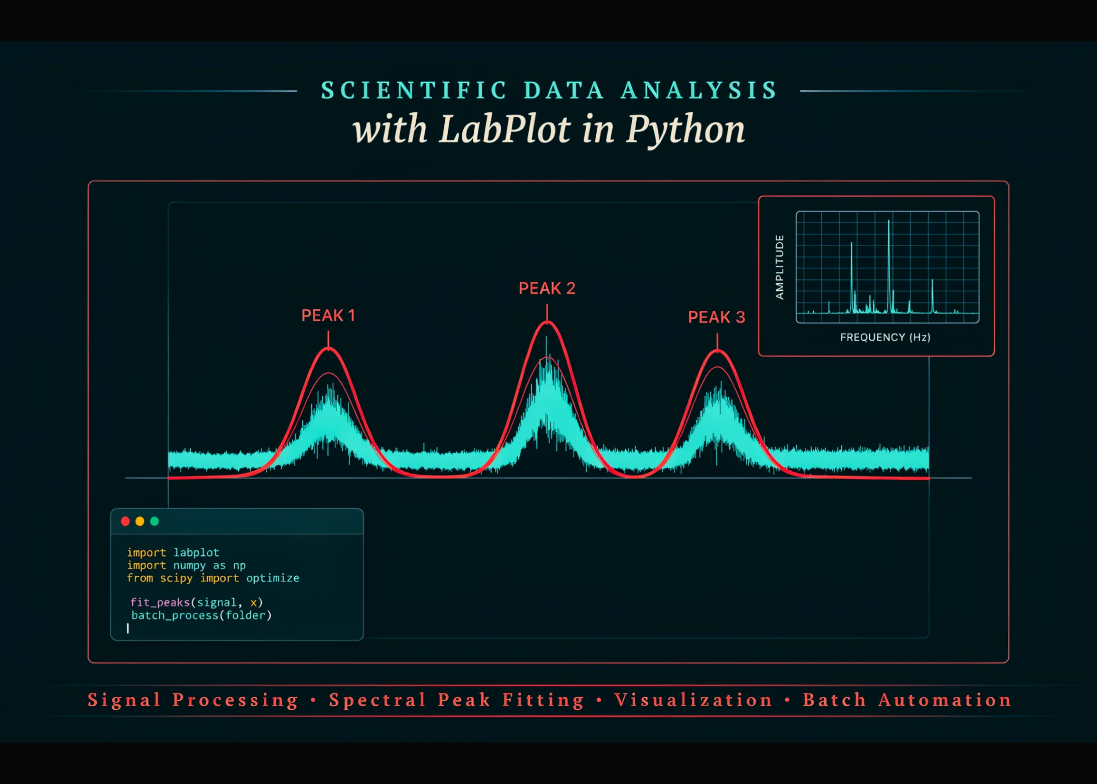
In this tutorial, we explore a LabPlot-inspired scientific data analysis workflow in Python while preserving the structure and terminology of LabPlot’s aspect tree, analysis kernels, plotting system, and project model. We build reusable components to import tabular data, compute descriptive statistics, smooth and differentiate signals, perform Fourier analysis and filtering, detect peaks, integrate curves, reduce data, and fit nonlinear models with detailed statistical diagnostics. We then apply these tools to a realistic spectroscopy example: removing periodic interference, identifying overlapping peaks, fitting a multi-Gaussian model, inspecting residuals, visualizing results through themed worksheets, exporting figures, and saving project data in LabPlot-compatible .lml-style files. Finally, we extend the same workflow to batch processing so we can analyze multiple temperature-dependent spectra and fit secondary trends across the resulting measurements.
import os, sys, gzip, bz2, lzma, time, math, textwrap, warnings import xml.etree.ElementTree as ET from dataclasses import dataclass, field from enum import Enum import numpy as np, pandas as pd, matplotlib, matplotlib.pyplot as plt from matplotlib.ticker import AutoMinorLocator import scipy from scipy import signal, stats, optimize warnings.filterwarnings("ignore", category=RuntimeWarning) np.random.seed(20260815) IN_COLAB = "google.colab" in sys.modules OUT = "https://www.marktechpost.com/content/labplot_out" if IN_COLAB else os.path.join(os.getcwd(), "labplot_out") os.makedirs(OUT, exist_ok=True) try: from pylabplot import *; HAVE_SDK = True except Exception: HAVE_SDK = False banner = lambda t: print("n" + "=" * 76 + f"n {t}n" + "=" * 76) banner("environment") print(f" numpy {np.__version__} | scipy {scipy.__version__} | mpl {matplotlib.__version__} | " f"colab={IN_COLAB} | pylabplot={'yes' if HAVE_SDK else 'no -> emulation'}n -> {OUT}") class PlotDesignation(Enum): NoDesignation = 0; X = 1; Y = 2; Z = 3 XError = 4; XErrorMinus = 5; XErrorPlus = 6 YError = 7; YErrorMinus = 8; YErrorPlus = 9 class ColumnMode(Enum): Double = 0; Text = 1; Integer = 2; BigInt = 3; DateTime = 4 class AbstractAspect: def __init__(self, name, comment=""): self._name, self.comment, self.parent, self.children = name, comment, None, [] def name(self): return self._name def addChild(self, a): a.parent = self; self.children.append(a); return a def tree(self, d=0): s = " " * d + f"{'|- ' if d else ''}{type(self).__name__:<20} {self._name}" if isinstance(self, Column): s += f" [{self.columnMode.name}, {self.rowCount()} rows, {self.plotDesignation.name}]" return "n".join([s] + [c.tree(d+1) for c in self.children]) class Column(AbstractAspect): """LabPlot's fundamental data source: a typed vector + a plot designation.""" def __init__(self, name, values=None, mode=ColumnMode.Double, designation=PlotDesignation.NoDesignation): super().__init__(name) self.columnMode, self.plotDesignation = mode, designation self._d = np.asarray([] if values is None else values, float) def values(self): return self._d def rowCount(self): return len(self._d) def clean(self): return self._d[np.isfinite(self._d)] def statistics(self): """The 20 quantities in LabPlot's Column Statistics dialog.""" x = self.clean(); n = x.size if not n: return {} q1, med, q3 = np.percentile(x, [25, 50, 75]); iqr, pos = q3 - q1, x[x > 0] h = 2 * iqr / n**(1/3) if iqr > 0 else 0 c, _ = np.histogram(x, bins=int(np.clip(np.ptp(x)/h, 1, 1000)) if h else 10) p = c[c > 0] / c.sum(); v, k = np.unique(np.round(x, 12), return_counts=True) return {"Count": n, "Minimum": x.min(), "Maximum": x.max(), "Arithmetic mean": x.mean(), "Geometric mean": stats.gmean(pos) if pos.size else np.nan, "Harmonic mean": stats.hmean(pos) if pos.size else np.nan, "Contraharmonic mean": (x**2).sum() / x.sum() if x.sum() else np.nan, "Mode": v[k.argmax()] if k.max() > 1 else np.nan, "First quartile": q1, "Median": med, "Third quartile": q3, "Interquartile range": iqr, "Trimean": (q1 + 2*med + q3) / 4, "Variance": x.var(ddof=1), "Standard deviation": x.std(ddof=1), "Skewness": stats.skew(x), "Mean absolute deviation": np.abs(x - x.mean()).mean(), "Median absolute deviation": np.median(np.abs(x - med)), "Kurtosis": stats.kurtosis(x, fisher=False), "Entropy": float(-(p * np.log2(p)).sum())} def sparkline(self, w=26): """LabPlot 2.11+ draws these in the column header; text version.""" b, x = "_.-~^", self.clean() s = x[np.linspace(0, x.size-1, min(w, x.size)).astype(int)] if x.size > 1 else x return "" if s.size < 2 or np.ptp(s) == 0 else "".join( b[i] for i in ((s - s.min()) / np.ptp(s) * 4).round().astype(int)) class Spreadsheet(AbstractAspect): def columns(self): return [c for c in self.children if isinstance(c, Column)] def column(self, k): cs = self.columns() return cs[k] if isinstance(k, int) else next(c for c in cs if c.name() == k) def columnCount(self): return len(self.columns()) def rowCount(self): return max([c.rowCount() for c in self.columns()], default=0) def appendColumn(self, n, v, d=PlotDesignation.Y): return self.addChild(Column(n, v, designation=d)) def toDataFrame(self): return pd.DataFrame({c.name(): c.values() for c in self.columns()}) def info(self): print(f" Spreadsheet '{self._name}': {self.rowCount()} rows x {self.columnCount()} cols") for c in self.columns(): s = c.statistics() print(f" {c.name():<12}{c.plotDesignation.name:<6}min {s['Minimum']:>9.4g} max " f"{s['Maximum']:>9.4g} mean {s['Arithmetic mean']:>9.4g} {c.sparkline()}") class Project(AbstractAspect): XML_VERSION = 15 def __init__(self, name="project", author=""): super().__init__(name); self.author, self.version = author, "2.12.1" def spreadsheets(self): return [c for c in self.children if isinstance(c, Spreadsheet)] class AsciiFilter: """LabPlot's text import: separator auto-detect, comments, row/col limits.""" def __init__(self, separator="auto", commentCharacter="#", headerEnabled=True, startRow=1, endRow=-1, startColumn=1, endColumn=-1): self.separator, self.commentCharacter = separator, commentCharacter self.headerEnabled, self.startRow, self.endRow = headerEnabled, startRow, endRow self.startColumn, self.endColumn = startColumn, endColumn def readDataFromFile(self, path, dataSource): with open(path, encoding="utf-8", errors="replace") as fh: lines = [l.rstrip("n") for l in fh if l.strip() and not l.lstrip().startswith(self.commentCharacter)] lines = lines[self.startRow - 1: None if self.endRow < 0 else self.endRow] if not lines: raise ValueError("AsciiFilter: nothing to import") sep = (next((s for s in (",", ";", "t", "|") if s in lines[0]), None) if self.separator == "auto" else self.separator) split = lambda l: [p.strip() for p in (l.split(sep) if sep else l.split()) if p.strip()] header = split(lines[0]) if self.headerEnabled else None rows = [split(l) for l in (lines[1:] if self.headerEnabled else lines)] ncol = max(map(len, rows)) c0, c1 = self.startColumn - 1, ncol if self.endColumn < 0 else self.endColumn for j in range(c0, min(c1, ncol)): vals = [] for r in rows: try: vals.append(float(r[j])) except (IndexError, ValueError): vals.append(np.nan) dataSource.addChild(Column( header[j] if header and j < len(header) else f"Column {j+1}", vals, designation=PlotDesignation.X if j == c0 else PlotDesignation.Y)) return dataSource We set up the Python environment, configure reproducibility, and establish the output directory for the tutorial. We recreate LabPlot’s core aspect-tree structure using projects, spreadsheets, columns, plot designations, and column modes. We also implement the AsciiFilter workflow to import structured text data into our LabPlot-style data model.
class nsl_smooth: """Analysis -> Smooth (Savitzky-Golay; LabPlot also offers moving average/percentile).""" @staticmethod def savitzky_golay(y, points=11, order=3, deriv=0): points += points % 2 == 0 return signal.savgol_filter(y, points, min(order, points-1), deriv=deriv, mode="interp") class nsl_diff: """Analysis -> Differentiate: order 1..6; SG differentiation for noisy data.""" @staticmethod def derive(x, y, order=1, smooth_points=0, sg_order=3): if smooth_points: return nsl_smooth.savitzky_golay(y, smooth_points, sg_order, deriv=order) / np.gradient(x) ** order out = np.asarray(y, float) for _ in range(order): out = np.gradient(out, x, edge_order=2) return out def simpson(x, y): """Composite Simpson on a non-uniform grid (Cartwright's formula).""" n = len(x) - 1 if n < 2: return float(np.trapezoid(y, x) if hasattr(np, "trapezoid") else np.trapz(y, x)) tot, i = 0.0, 0 while i + 2 <= n: h0, h1 = x[i+1] - x[i], x[i+2] - x[i+1]; hp, hd, hm = h1 + h0, h1 / h0, h1 * h0 tot += hp / 6 * ((2-hd) * y[i] + hp**2 / hm * y[i+1] + (2 - 1/hd) * y[i+2]); i += 2 return tot + ((x[n]-x[n-1]) * (y[n]+y[n-1]) / 2 if i < n else 0) class nsl_int: """Analysis -> Integrate: rectangle / trapezoid / Simpson, cumulative.""" @staticmethod def integrate(x, y, method="trapezoid", absolute=False): yy = np.abs(y) if absolute else np.asarray(y, float) seg = np.diff(x) * (yy[:-1] if method == "rectangle" else (yy[:-1] + yy[1:]) / 2) cum = np.r_[0.0, np.cumsum(seg)] return cum * simpson(x, yy) / cum[-1] if method == "simpson" and cum[-1] else cum class nsl_dft: """Analysis -> Fourier Transform: amplitude/magnitude/power/dB, 5 windows.""" WIN = {"rectangular": np.ones, "hann": lambda n: signal.windows.hann(n, sym=False), "hamming": lambda n: signal.windows.hamming(n, sym=False), "blackman": lambda n: signal.windows.blackman(n, sym=False), "flattop": lambda n: signal.windows.flattop(n, sym=False)} @staticmethod def transform(x, y, output="amplitude", window="rectangular"): n, dt = len(y), float(np.mean(np.diff(x))) w = nsl_dft.WIN[window](n); cg = w.mean() Y = np.fft.rfft(y * w); f = np.fft.rfftfreq(n, dt); m = np.abs(Y) v = {"magnitude": lambda: m, "power": lambda: m**2 / (n*cg)**2, "phase": lambda: np.angle(Y), "amplitude": lambda: np.r_[m[0]/(n*cg), 2*m[1:]/(n*cg)], "dB": lambda: 20*np.log10(np.maximum(m / (m.max() or 1), 1e-16))}[output]() return f, v class nsl_filter: """Analysis -> Fourier Filter: low/high/band pass + band reject; ideal or Butterworth.""" @staticmethod def apply(x, y, type="lowpass", form="butterworth", cutoff=.1, cutoff2=.3, order=3): n = len(y); f = np.fft.rfftfreq(n, float(np.mean(np.diff(x)))); eps = 1e-30 if type == "lowpass": r = f / cutoff elif type == "highpass": r = cutoff / np.maximum(f, eps) else: f0, bw = math.sqrt(cutoff * cutoff2), cutoff2 - cutoff r = np.abs((f**2 - f0**2) / np.maximum(f * bw, eps)) if type == "bandreject": r = 1 / np.maximum(r, eps) H = (r <= 1).astype(float) if form == "ideal" else 1 / np.sqrt(1 + r ** (2 * order)) return np.fft.irfft(np.fft.rfft(y) * H, n=n) class nsl_hilbert: """Analysis -> Hilbert Transform (LabPlot 2.9+).""" @staticmethod def transform(y, output="envelope"): a = signal.hilbert(y) return {"imag": a.imag, "real": a.real, "envelope": np.abs(a), "phase": np.unwrap(np.angle(a))}[output] class nsl_geom: """Analysis -> Data Reduction: Douglas-Peucker, iterative (no recursion limit).""" @staticmethod def douglas_peucker(x, y, tol): n = len(x); keep = np.zeros(n, bool); keep[[0, -1]] = True; stack = [(0, n-1)] while stack: i, j = stack.pop() if j <= i + 1: continue dx, dy = x[j]-x[i], y[j]-y[i]; den = math.hypot(dx, dy); sl = slice(i+1, j) d = (np.hypot(x[sl]-x[i], y[sl]-y[i]) if den == 0 else np.abs(dy*(x[sl]-x[i]) - dx*(y[sl]-y[i])) / den) if d.size and d.max() > tol: k = i + 1 + int(d.argmax()); keep[k] = True; stack += [(i, k), (k, j)] return np.flatnonzero(keep) class nsl_peak: """Analysis -> Peak Find (LabPlot 2.11+); seeds multi-peak fits.""" @staticmethod def find(x, y, prominence=None, distance=None): pk, pr = signal.find_peaks(y, prominence=prominence, distance=distance) w = signal.peak_widths(y, pk, rel_height=.5)[0] if pk.size else np.array([]) return pk, {"positions": x[pk], "heights": y[pk], "prominences": pr.get("prominences", np.array([])), "fwhm": w * float(np.mean(np.diff(x)))} class nsl_fit_model: """LabPlot's model catalogue (Basic / Peak / Growth / Distribution).""" @staticmethod def gaussian(x, a, mu, s): return a / (math.sqrt(2 * np.pi) * s) * np.exp(-(x - mu) ** 2 / (2 * s ** 2)) @staticmethod def lorentz(x, a, mu, g): return a / np.pi * (g / 2) / ((x - mu) ** 2 + (g / 2) ** 2) @dataclass class FitResult: names: list; values: np.ndarray; errors: np.ndarray; t: np.ndarray; p: np.ndarray margin: np.ndarray; gof: dict; dof: int; nfev: int; status: str elapsed: float; unweighted: bool residuals: np.ndarray = field(repr=False, default=None) cov: np.ndarray = field(repr=False, default=None) def report(self, title="Fit result"): print(f"n{'-'*76}n {title}n{'-'*76}") print(f" {self.status} | nfev {self.nfev} | dof {self.dof} | {self.elapsed*1e3:.1f} ms") print(f"n {'param':<8}{'value':>13}{'error':>11}{'err%':>8}{'t':>8}{'P>|t|':>10}{'95% CI':>26}") for i, n in enumerate(self.names): v, e, m = self.values[i], self.errors[i], self.margin[i] print(f" {n:<8}{v:>13.6g}{e:>11.4g}{abs(100*e/v) if v else np.inf:>7.2f}%" f"{self.t[i]:>8.1f}{self.p[i]:>10.2g}{f'[{v-m:.5g},{v+m:.5g}]':>26}") print("n goodness of fit") it = list(self.gof.items()) for i in range(0, len(it), 2): r = f"{it[i+1][0]:<22}{it[i+1][1]:>14.6g}" if i + 1 < len(it) else "" print(f" {it[i][0]:<22}{it[i][1]:>14.6g} {r}") if self.unweighted: print(" note: no y-errors given, so chi^2 == SSE and 'P > chi^2' is not a realn" " test. Pass yerr= for a meaningful reduced chi^2.") print("-" * 76) class nsl_fit: @staticmethod def fit(model, x, y, p0, yerr=None, bounds=None, paramNames=None, conf=.95): """GSL's multifit_nlinear == scipy least_squares(method='lm').""" t0 = time.perf_counter() x, y, p0 = np.asarray(x, float), np.asarray(y, float), np.asarray(p0, float) sig = np.ones_like(y) if yerr is None else np.asarray(yerr, float) res = lambda p: (model(x, *p) - y) / sig kw = dict(max_nfev=500*len(p0), **({"method": "lm"} if bounds is None else {"bounds": bounds})) out = optimize.least_squares(res, p0, **kw) p = out.x; n, k = len(y), len(p); dof = max(n - k, 1); r = y - model(x, *p) sse = float((r**2).sum()); chisq = float(((r / sig)**2).sum()); red = chisq / dof try: cov = np.linalg.inv(out.jac.T @ out.jac) except np.linalg.LinAlgError: cov = np.linalg.pinv(out.jac.T @ out.jac) cov = cov * (red if yerr is None else 1.0); err = np.sqrt(np.abs(np.diag(cov))) tv = np.divide(p, err, out=np.full_like(p, np.inf), where=err > 0) sst = float(((y - y.mean())**2).sum()); r2 = 1 - sse/sst if sst else np.nan F = (r2 / max(k-1, 1)) / ((1-r2) / dof) if r2 < 1 else np.inf logL = -.5*n * (math.log(2*math.pi) + math.log(sse/n) + 1); aic = 2*k - 2*logL gof = {"sum sq. residuals": sse, "mean squared error": sse/n, "root MSE": math.sqrt(sse/n), "mean abs. error": float(np.abs(r).mean()), "residual std dev": math.sqrt(sse/dof), "R^2": r2, "adjusted R^2": 1 - (1-r2)*(n-1)/dof, "chi^2": chisq, "reduced chi^2": red, "P > chi^2": stats.chi2.sf(chisq, dof), "F statistic": F, "P > F": stats.f.sf(F, max(k-1, 1), dof), "log-likelihood": logL, "AIC": aic, "AICc": aic + 2*k*(k+1)/max(n-k-1, 1), "BIC": k*math.log(n) - 2*logL} return FitResult(paramNames or [f"p{i}" for i in range(k)], p, err, tv, 2 * stats.t.sf(np.abs(tv), dof), stats.t.ppf(.5 + conf/2, dof) * err, gof, dof, int(out.nfev), out.message, time.perf_counter() - t0, yerr is None, r, cov) @staticmethod def confidenceBand(model, x, res, level=.95, eps=1e-7): """Delta method sqrt(diag(J C J^T)) * t -- LabPlot's CI overlay.""" p = res.values; J = np.empty((len(x), len(p))) for i in range(len(p)): dp = np.zeros_like(p); dp[i] = eps * max(abs(p[i]), 1) J[:, i] = (model(x, *(p + dp)) - model(x, *(p - dp))) / (2 * dp[i]) v = np.einsum("ij,jk,ik->i", J, res.cov, J) return stats.t.ppf(.5 + level/2, res.dof) * np.sqrt(np.maximum(v, 0)) @staticmethod def distributionFitML(data, dist="norm"): """nsl_fit_algorithm_ml -- max-likelihood distribution fit (the SDK demo).""" d = getattr(stats, dist); pr = d.fit(data); ks = stats.kstest(data, dist, args=pr) ll = float(d.logpdf(data, *pr).sum()) return {"params": pr, "logLik": ll, "AIC": 2 * len(pr) - 2 * ll, "KS_stat": ks.statistic, "KS_p": ks.pvalue, "pdf": lambda t: d.pdf(t, *pr)} We implement the main numerical analysis kernels that let us smooth, differentiate, integrate, transform, filter, reduce, and inspect scientific signals. We add peak detection along with Gaussian and Lorentzian models for advanced curve analysis. We also build nonlinear fitting utilities that calculate parameter uncertainties, confidence intervals, goodness-of-fit statistics, and maximum-likelihood distribution fits.
THEMES = { "BlackOnWhite": dict(bg="#ffffff", fg="#000000", grid="#c8c8c8", cycle=["#3465a4", "#cc0000", "#4e9a06", "#f57900", "#75507b", "#06989a"]), "Dracula": dict(bg="#282a36", fg="#f8f8f2", grid="#44475a", cycle=["#8be9fd", "#ff79c6", "#50fa7b", "#ffb86c", "#bd93f9", "#f1fa8c"]), "SolarizedDark": dict(bg="#002b36", fg="#93a1a1", grid="#0f4b57", cycle=["#268bd2", "#dc322f", "#859900", "#b58900", "#6c71c4", "#2aa198"])} class XYCurve(AbstractAspect): def __init__(self, name, x=None, y=None, lineStyle="-", lineWidth=1.6, symbolStyle=None, symbolSize=4., color=None, alpha=1., zorder=2): super().__init__(name) self.xColumn, self.yColumn, self.color, self.alpha = x, y, color, alpha self.lineStyle, self.lineWidth = lineStyle, lineWidth self.symbolStyle, self.symbolSize, self.zorder = symbolStyle, symbolSize, zorder self.yErrorColumn = self.fillBetween = None def setXColumn(self, c): self.xColumn = c; return self def setYColumn(self, c): self.yColumn = c; return self @staticmethod def _v(c): return c.values() if isinstance(c, Column) else np.asarray(c, float) def draw(self, ax, color): c = self.color or color; X, Y = self._v(self.xColumn), self._v(self.yColumn) if self.fillBetween is not None: ax.fill_between(X, *self.fillBetween, color=c, alpha=.2, lw=0, zorder=self.zorder-1) if self.yErrorColumn is not None: ax.errorbar(X, Y, yerr=self._v(self.yErrorColumn), fmt="none", ecolor=c, elinewidth=.8, capsize=2, alpha=.7, zorder=self.zorder) ax.plot(X, Y, linestyle=self.lineStyle or "none", marker=self.symbolStyle or "none", markersize=self.symbolSize, linewidth=self.lineWidth, color=c, alpha=self.alpha, label=self._name, zorder=self.zorder, markeredgewidth=0) class Histogram(AbstractAspect): """normalization: 'Count' | 'Probability' | 'CountDensity' | 'ProbabilityDensity'.""" def __init__(self, name, dataColumn=None, bins="auto", normalization="ProbabilityDensity"): super().__init__(name) self.dataColumn, self.bins, self.normalization = dataColumn, bins, normalization def draw(self, ax, color): d = (self.dataColumn.clean() if isinstance(self.dataColumn, Column) else np.asarray(self.dataColumn, float)) ax.hist(d, bins=self.bins, color=color, alpha=.55, edgecolor=color, lw=.8, label=self._name, zorder=1, density="Density" in self.normalization or self.normalization == "Probability") class CartesianPlot(AbstractAspect): class Type(Enum): FourAxes = 0; TwoAxes = 1 def __init__(self, name, title=None, xLabel="x", yLabel="y", logX=False, logY=False): super().__init__(name); self.type = CartesianPlot.Type.FourAxes self.title, self.xLabel, self.yLabel = title or name, xLabel, yLabel self.logX, self.logY, self.legend = logX, logY, None self.xRange, self.yRange, self.labels = None, None, [] def setType(self, t): self.type = t; return self def addLegend(self, loc="best"): self.legend = loc; return self def setRange(self, x=None, y=None): self.xRange, self.yRange = x, y; return self def addTextLabel(self, txt, x, y): self.labels.append((txt, x, y)); return self def _render(self, ax, th): ax.set_facecolor(th["bg"]) for i, ch in enumerate(self.children): ch.draw(ax, th["cycle"][i % len(th["cycle"])]) ax.set_title(self.title, color=th["fg"], fontsize=10.5, pad=7) ax.set_xlabel(self.xLabel, color=th["fg"], fontsize=9.5) ax.set_ylabel(self.yLabel, color=th["fg"], fontsize=9.5) for lg, sc, axis in ((self.logX, ax.set_xscale, ax.xaxis), (self.logY, ax.set_yscale, ax.yaxis)): sc("log") if lg else axis.set_minor_locator(AutoMinorLocator(2)) if self.xRange: ax.set_xlim(*self.xRange) if self.yRange: ax.set_ylim(*self.yRange) four = self.type is CartesianPlot.Type.FourAxes for s in ("top", "right"): ax.spines[s].set_visible(four) for s in ax.spines.values(): s.set_color(th["fg"]); s.set_linewidth(.9) ax.tick_params(which="both", direction="in", colors=th["fg"], top=four, right=four, labelsize=8.5) ax.grid(True, color=th["grid"], lw=.6, alpha=.7, zorder=0) for t, x, y in self.labels: ax.annotate(t, (x, y), color=th["fg"], fontsize=7.5, ha="center") if self.legend: for t in ax.legend(loc=self.legend, fontsize=8, framealpha=.85, facecolor=th["bg"], edgecolor=th["grid"]).get_texts(): t.set_color(th["fg"]) class Worksheet(AbstractAspect): class ExportFormat(Enum): PDF = 0; SVG = 1; PNG = 2 def __init__(self, name, cols=None, figsize=(15, 8.5), dpi=110): super().__init__(name); self.themeName = "BlackOnWhite" self.cols, self.figsize, self.dpi, self._fig = cols, figsize, dpi, None def setTheme(self, n): if n not in THEMES: raise KeyError(f"themes: {list(THEMES)}") self.themeName = n; return self def render(self): th = THEMES[self.themeName] ps = [c for c in self.children if isinstance(c, CartesianPlot)] cols = self.cols or min(len(ps), 2) fig, axes = plt.subplots(math.ceil(len(ps)/cols), cols, figsize=self.figsize, dpi=self.dpi) fig.patch.set_facecolor(th["bg"]); axes = np.atleast_1d(axes).ravel() for ax, p in zip(axes, ps): p._render(ax, th) for ax in axes[len(ps):]: ax.axis("off") fig.suptitle(self._name, color=th["fg"], fontsize=13, y=.995) fig.tight_layout(rect=(0, 0, 1, .98)); self._fig = fig; return fig def show(self): (self.render() if self._fig is None else None); plt.show() def exportToFile(self, path, format=None): if self._fig is None: self.render() fmt = (format.name.lower() if isinstance(format, Worksheet.ExportFormat) else format or os.path.splitext(path)[1].lstrip(".")) self._fig.savefig(path, format=fmt, dpi=self.dpi, bbox_inches="tight", facecolor=self._fig.get_facecolor()); return path def _reduce(x, y, tolerance=None): i = nsl_geom.douglas_peucker(x, y, tolerance if tolerance is not None else .02*np.ptp(y)) return x[i], y[i], {"in": len(x), "out": len(i), "compression": 1 - len(i)/len(x)} class XYAnalysisCurve(XYCurve): OPS = { "smooth": lambda x, y, points=11, order=3: (x, nsl_smooth.savitzky_golay(y, points, order), {}), "differentiate": lambda x, y, derivOrder=1, smoothPoints=0: (x, nsl_diff.derive(x, y, derivOrder, smoothPoints), {}), "integrate": lambda x, y, method="trapezoid", absolute=False: (lambda c: (x, c, {"total": float(c[-1])}))(nsl_int.integrate(x, y, method, absolute)), "dft": lambda x, y, output="amplitude", window="rectangular": nsl_dft.transform(x, y, output, window) + ({},), "filter": lambda x, y, type="lowpass", form="butterworth", cutoff=.1, cutoff2=.3, order=3: (x, nsl_filter.apply(x, y, type, form, cutoff, cutoff2, order), {}), "hilbert": lambda x, y, output="envelope": (x, nsl_hilbert.transform(y, output), {}), "reduce": _reduce} def __init__(self, name, xData, yData, op, style=None, **opts): super().__init__(name, **(style or {})) self._xin, self._yin = XYCurve._v(xData), XYCurve._v(yData) self.op, self.opts, self.result = op, opts, None self.recalculate() def recalculate(self): self.xColumn, self.yColumn, self.result = XYAnalysisCurve.OPS[self.op](self._xin, self._yin, **self.opts) return self _mk = lambda op: (lambda name, x, y, style=None, **kw: XYAnalysisCurve(name, x, y, op, style, **kw)) XYSmoothCurve, XYDifferentiationCurve = _mk("smooth"), _mk("differentiate") XYIntegrationCurve = _mk("integrate") XYFourierTransformCurve, XYFourierFilterCurve = _mk("dft"), _mk("filter") XYHilbertTransformCurve, XYDataReductionCurve = _mk("hilbert"), _mk("reduce") class XYFitCurve(XYCurve): """LabPlot's centrepiece: non-linear fitting with the full statistics table.""" def __init__(self, name, xData, yData, model, p0, paramNames=None, yerr=None, bounds=None, npoints=800, **kw): super().__init__(name, **kw) self._xin, self._yin = XYCurve._v(xData), XYCurve._v(yData) self.model, self.p0, self.paramNames = model, p0, paramNames self.yerr, self.bounds, self.npoints, self.fitResult = yerr, bounds, npoints, None def recalculate(self, conf=.95, showConfidenceInterval=True): self.fitResult = nsl_fit.fit(self.model, self._xin, self._yin, self.p0, self.yerr, self.bounds, self.paramNames, conf) xf = np.linspace(self._xin.min(), self._xin.max(), self.npoints) yf = self.model(xf, *self.fitResult.values); self.xColumn, self.yColumn = xf, yf if showConfidenceInterval: d = nsl_fit.confidenceBand(self.model, xf, self.fitResult, conf) self.fillBetween = (yf - d, yf + d) return self class ProjectFile: MAGIC = ((b"x1fx8b", gzip.decompress, "gzip"), (b"BZh", bz2.decompress, "bzip2"), (b"xfd7zXZx00", lzma.decompress, "xz")) @staticmethod def load(path): blob = open(path, "rb").read(); kind = "plain" for magic, dec, nm in ProjectFile.MAGIC: if blob.startswith(magic): blob, kind = dec(blob), nm; break root = ET.fromstring(blob.decode("utf-8", "replace")) root = root if root.tag == "project" else root.find(".//project") if root is None: raise ValueError("no project element found") prj = Project(os.path.basename(path), root.get("author", "")) prj.version = root.get("version", "?") print(f" loaded .lml: compression={kind} version={prj.version} xmlVersion=" f"{root.get('xmlVersion','?')}") parents = {c: p for p in root.iter() for c in p} def sheet_of(n): n = parents.get(n) while n is not None and n.tag != "spreadsheet": n = parents.get(n) return n buckets = {} for col in root.iter("column"): buckets.setdefault(id(sheet_of(col)), (sheet_of(col), []))[1].append(col) for el, cols in buckets.values(): sp = Spreadsheet(el.get("name", "spreadsheet") if el is not None else "sheet") for c in cols: sp.addChild(ProjectFile._column(c)) prj.addChild(sp) return prj @staticmethod def _column(el): name = el.get("name") or next( (el.find(t).get("name") for t in ("general", "comment") if el.find(t) is not None and el.find(t).get("name")), "Column") rows = el.findall("row") if rows: raw = [r.text for r in sorted(rows, key=lambda r: int(r.get("index", 0)))] else: node = next((el.find(t) for t in ("values", "data", "double") if el.find(t) is not None and el.find(t).text), None) raw = (node.text if node is not None else el.text or "").split() vals = [] for v in raw: try: vals.append(float(v)) except (TypeError, ValueError): vals.append(np.nan) try: des = PlotDesignation(int(el.get("designation", 0))) except (ValueError, TypeError): des = PlotDesignation.NoDesignation return Column(name, vals, designation=des) @staticmethod def save(project, path, compression="gzip"): root = ET.Element("project", { "version": project.version, "xmlVersion": str(Project.XML_VERSION), "fileName": os.path.basename(path), "author": project.author, "modificationTime": time.strftime("%Y-%m-%d %H:%M:%S")}) ET.SubElement(root, "comment").text = project.comment for sp in project.spreadsheets(): e = ET.SubElement(root, "spreadsheet", {"name": sp.name()}) ET.SubElement(e, "general", {"rowCount": str(sp.rowCount()), "columnCount": str(sp.columnCount())}) for col in sp.columns(): c = ET.SubElement(e, "column", { "name": col.name(), "rows": str(col.rowCount()), "designation": str(col.plotDesignation.value), "mode": str(col.columnMode.value)}) for i, v in enumerate(col.values()): ET.SubElement(c, "row", {"index": str(i)}).text = repr(float(v)) xml = (b'nn' + ET.tostring(root, encoding="utf-8")) open(path, "wb").write({"gzip": gzip.compress, "bzip2": bz2.compress, "xz": lzma.compress, "none": lambda b: b}[compression](xml)) return path We construct the visualization layer using curves, histograms, Cartesian plots, worksheets, themes, and reusable analysis-curve objects. We connect these plotting objects directly to our numerical operations so we can recalculate processed curves and fitted models programmatically. We also implement LabPlot-style project file loading and saving, including compressed .lml formats and spreadsheet reconstruction.
banner("STEP 1 import an instrument file with AsciiFilter") wl = np.linspace(400., 700., 1500) TRUE = [(120., 468., 6.), (75., 512., 4.5), (140., 545., 9.), (55., 604., 5.)] clean = 18. - .012 * (wl - 400) for a, mu, s in TRUE: clean = clean + nsl_fit_model.gaussian(wl, a, mu, s) counts = clean + 2.2 * np.sin(2*np.pi * wl / 3.7) + np.random.normal(0, 1.1, wl.size) raw = os.path.join(OUT, "spectrum.dat") with open(raw, "w") as fh: fh.write("# SpecMaster-9000, 500 ms integrationnwavelengthtcountsn") fh.writelines(f"{a:.4f}t{b:.5f}n" for a, b in zip(wl, counts)) project = Project("spectroscopy demo", "LabPlot Colab tutorial") data = project.addChild(Spreadsheet("data")) AsciiFilter().readDataFromFile(raw, data) x, y = data.column("wavelength"), data.column("counts") data.info() banner("STEP 2 column statistics") it = list(y.statistics().items()) for i in range(0, len(it), 2): print(f" {it[i][0]:<26}{it[i][1]:>13.6g} " + (f"{it[i+1][0]:<26}{it[i+1][1]:>13.6g}" if i + 1 < len(it) else "")) banner("STEP 3-4 FFT finds the fringe; a band-reject notch removes it") freq, amp = nsl_dft.transform(x.values(), y.values(), "amplitude", "hann") i0 = int(np.argmax(amp[5:])) + 5; f0 = freq[i0] print(f" dominant component {f0:.4f} 1/nm -> period {1/f0:.3f} nm (injected 3.700), " f"amplitude {amp[i0]:.3f} (injected 2.200)") yf = XYFourierFilterCurve("fringe removed", x, y, type="bandreject", form="butterworth", cutoff=f0*.82, cutoff2=f0*1.22, order=6).yColumn print(f" notch {f0*.82:.3f}-{f0*1.22:.3f} 1/nm | residual std vs truth " f"{np.std(y.values()-clean):.3f} -> {np.std(yf-clean):.3f}") banner("STEP 5 smooth + 2nd derivative -> locate peaks objectively") smooth = XYSmoothCurve("SG smoothed", x, yf, points=41, order=3) d2 = XYDifferentiationCurve("2nd derivative", x, smooth.yColumn, derivOrder=2, smoothPoints=61) pk, pr = nsl_peak.find(x.values(), -d2.yColumn, prominence=np.ptp(d2.yColumn)*.20, distance=25) print(f" {len(pk)} peaks in -y'' | found " + ", ".join(f"{v:7.2f}" for v in pr["positions"]) + "n | truth " + ", ".join(f"{t[1]:7.2f}" for t in TRUE)) banner("STEP 6 non-linear multi-peak fit (Levenberg-Marquardt)") NPEAK = 4 centres = np.sort(pr["positions"][np.argsort(pr["heights"])[::-1][:NPEAK]]) def multi_gauss(xx, c0, c1, *p): """Linear baseline + NPEAK Gaussians -- the 'Custom' model you'd type in.""" out = c0 + c1 * xx for i in range(NPEAK): out = out + nsl_fit_model.gaussian(xx, *p[3*i:3*i+3]) return out p0 = [18., -.012] for mu in centres: j = int(np.argmin(np.abs(x.values() - mu))) p0 += [max(smooth.yColumn[j] - 12, 5.) * 15., float(mu), 6.] names = ["b0", "b1"] + sum([[f"A{i+1}", f"mu{i+1}", f"sg{i+1}"] for i in range(NPEAK)], []) lo = [-np.inf, -np.inf] + sum([[0., m - 12, .5] for m in centres], []) hi = [np.inf, np.inf] + sum([[np.inf, m + 12, 40.] for m in centres], []) fit = XYFitCurve("fit + 95% CI", x, yf, multi_gauss, p0, names, bounds=(lo, hi), lineWidth=2.) fit.recalculate() fit.fitResult.report("XYFitCurve :: 4 Gaussians + linear baseline") pv = fit.fitResult.values print(f"n {'peak':<6}{'area':>10}{'true':>8}{'centre':>11}{'true':>9}{'sigma':>9}{'true':>8}") for i, (a, mu, s) in enumerate(TRUE): print(f" {i+1:<6}{pv[2+3*i]:>10.2f}{a:>8.1f}{pv[3+3*i]:>11.3f}{mu:>9.1f}{pv[4+3*i]:>9.3f}{s:>8.1f}") banner("STEP 7 integration, data reduction, Hilbert envelope") base = pv[0] + pv[1] * x.values(); net = yf - base tot = XYIntegrationCurve("cumulative", x, net, method="simpson") print(f" total net signal (Simpson) {tot.result['total']:.2f}; per-peak analytic vs numeric:") for i, (a, mu, s) in enumerate(TRUE): A, M, S = pv[2+3*i], pv[3+3*i], pv[4+3*i]; m = np.abs(x.values() - M) < 3.5 * S print(f" peak {i+1}: {A:7.2f} vs {simpson(x.values()[m], net[m]):7.2f} (true {a:.0f})") print(" peaks 2/3 overlap, so their numeric windows double-count the shared area -- whichn" " is exactly why you fit a multi-peak model instead of integrating windows by hand.") red = XYDataReductionCurve("reduced", x, smooth.yColumn, tolerance=.4) err = np.max(np.abs(np.interp(x.values(), red.xColumn, red.yColumn) - smooth.yColumn)) env = XYHilbertTransformCurve("envelope", x, y.values() - smooth.yColumn) print(f" Douglas-Peucker tol=0.4: {red.result['in']} -> {red.result['out']} pts " f"({red.result['compression']*100:.1f}% dropped), max error {err:.4f}n" f" Hilbert envelope of the removed fringe: mean {env.yColumn.mean():.3f} counts" f" (injected amplitude 2.200)") banner("STEP 8 residual diagnostics") res = fit.fitResult.residuals ml = nsl_fit.distributionFitML(res, "norm") dw = float(np.sum(np.diff(res)**2) / np.sum(res**2)) print(f" ML normal mu={ml['params'][0]:+.4f} sigma={ml['params'][1]:.4f} AIC={ml['AIC']:.1f}n" f" KS D={ml['KS_stat']:.4f} p={ml['KS_p']:.4f} | Shapiro W=" f"{stats.shapiro(res[:5000]).statistic:.4f} | Durbin-Watson d={dw:.3f}n -> " f"{'consistent with white Gaussian noise' if ml['KS_p']>.05 and 1.5We generate a realistic noisy spectroscopy dataset containing a sloping baseline, overlapping Gaussian peaks, periodic interference, and random noise. We use Fourier analysis, band-reject filtering, smoothing, differentiation, and peak detection to isolate key spectral features before fitting. We then perform a constrained multi-Gaussian fit, integrate the recovered signal, reduce the data, calculate a Hilbert envelope, and statistically evaluate the fit residuals.
banner("STEP 9 Worksheet -> CartesianPlots -> theme -> export") ws = Worksheet("Spectroscopy analysis", cols=3, figsize=(15, 8.5)) ws.setTheme("Dracula") p1 = CartesianPlot("raw & fit", "Raw spectrum + multi-Gaussian fit", "wavelength (nm)", "counts") p1.addLegend("upper right").addChild(XYCurve("raw", x, y, lineWidth=.6, alpha=.45)) p1.addChild(XYCurve("fringe removed", x, yf, lineWidth=.9, alpha=.8)); p1.addChild(fit) p2 = CartesianPlot("components", "Resolved components", "wavelength (nm)", "counts") p2.addLegend("upper right").addChild(XYCurve("baseline", x, base, lineStyle="--", lineWidth=1.2)) for i in range(NPEAK): A, M, S = pv[2+3*i], pv[3+3*i], pv[4+3*i] p1.addTextLabel(f"{M:.1f}", M, multi_gauss(M, *pv) + 1.2) p2.addChild(XYCurve(f"peak {i+1} ({M:.1f} nm)", x, base + nsl_fit_model.gaussian(x.values(), A, M, S), lineWidth=1.3)) f2, a2 = nsl_dft.transform(x.values(), yf, "amplitude", "hann") p3 = CartesianPlot("fft", "Amplitude spectrum (Hann)", "spatial frequency (1/nm)", "amplitude", logY=True).addLegend("upper right").setRange(x=(0, .6)) p3.addChild(XYCurve("raw", freq, np.maximum(amp, 1e-4), lineWidth=1.)) p3.addChild(XYCurve("filtered", f2, np.maximum(a2, 1e-4), lineWidth=1.)) p3.addTextLabel(f"fringen{f0:.3f} 1/nm", f0, amp[i0] * 1.6) p4 = CartesianPlot("d2", "Second derivative (peak detection)", "wavelength (nm)", "d2(counts)/dx2") p4.addLegend("lower right").addChild(XYCurve("-y''", x, -d2.yColumn, lineWidth=1.)) p4.addChild(XYCurve("detected", x.values()[pk], -d2.yColumn[pk], lineStyle=None, symbolStyle="o", symbolSize=6.)) tt = np.linspace(res.min(), res.max(), 400) p5 = CartesianPlot("residuals", "Fit residuals + ML normal", "residual (counts)", "probability density").addLegend("upper right") p5.addChild(Histogram("residuals", res, bins=45)) p5.addChild(XYCurve(f"N({ml['params'][0]:.2f}, {ml['params'][1]:.2f})", tt, ml["pdf"](tt), lineWidth=2.)) for p in (p1, p2, p3, p4, p5): ws.addChild(p) ws.render() for ext, f in ((".png", None), (".pdf", Worksheet.ExportFormat.PDF), (".svg", Worksheet.ExportFormat.SVG)): ws.exportToFile(os.path.join(OUT, "worksheet" + ext), f) print(" exported worksheet.png / .pdf / .svg"); ws.show() banner("STEP 10 project tree + .lml round-trip") r = project.addChild(Spreadsheet("analysis results")) r.appendColumn("wavelength", x.values(), PlotDesignation.X) for n, v in (("filtered", yf), ("smoothed", smooth.yColumn), ("baseline", base), ("fit", multi_gauss(x.values(), *pv)), ("residuals", yf - multi_gauss(x.values(), *pv)), ("cumulative", tot.yColumn)): r.appendColumn(n, v) pp = project.addChild(Spreadsheet("fit parameters")) pp.appendColumn("value", pv) pp.appendColumn("error", fit.fitResult.errors, PlotDesignation.YError) project.addChild(ws) print(project.tree()) for c, ext in (("gzip", ".lml.gz"), ("xz", ".lml.xz"), ("none", ".lml")): f = ProjectFile.save(project, os.path.join(OUT, "spectroscopy" + ext), c) print(f" saved {os.path.basename(f):<24}{os.path.getsize(f)/1024:>8.1f} kB ({c})") back = ProjectFile.load(os.path.join(OUT, "spectroscopy.lml.gz")) o, b = y.values(), back.spreadsheets()[0].column("counts").values() print(f" round-trip: max |delta| = {np.max(np.abs(o-b)):.3e} {'OK' if np.allclose(o,b) else 'BAD'}") r.toDataFrame().to_csv(os.path.join(OUT, "analysis_results.csv"), index=False) We organize the spectroscopy results into a themed worksheet containing the raw spectrum, fitted components, Fourier spectrum, detected peaks, and residual distribution. We export the complete visualization to PNG, PDF, and SVG formats so we have reusable graphical outputs. We also store our processed measurements and fitted parameters inside the project, save them in several .lml formats, and verify that the project data survives a complete round trip.
banner("STEP 11 batch: import -> filter -> fit -> secondary fit") bd = os.path.join(OUT, "batch"); os.makedirs(bd, exist_ok=True) temps = [20, 40, 60, 80, 100, 120] for T in temps: yy = 18. - .012 * (wl - 400) for a, mu, s in TRUE: yy = yy + nsl_fit_model.gaussian(wl, a * math.exp(-(T-20)/140), mu + .045*(T-20), s * (1 + .004*(T-20))) with open(os.path.join(bd, f"run_{T:03d}C.dat"), "w") as fh: fh.write(f"# T = {T} Cnwavelengthtcountsn") fh.writelines(f"{a:.4f}t{b:.5f}n" for a, b in zip(wl, yy + np.random.normal(0, 1.1, wl.size))) def analyse(path): sp = Spreadsheet(os.path.basename(path)); AsciiFilter().readDataFromFile(path, sp) q = XYFitCurve("fit", sp.column(0), sp.column(1), multi_gauss, p0, names, bounds=(lo, hi)) .recalculate(showConfidenceInterval=False).fitResult return {"file": os.path.basename(path), "area": q.values[8], "area_err": q.errors[8], "centre": q.values[9], "centre_err": q.errors[9], "R2": q.gof["R^2"]} t0 = time.perf_counter() df = pd.DataFrame([analyse(os.path.join(bd, f)) for f in sorted(os.listdir(bd))]) df.insert(1, "T_C", temps) print(df.to_string(index=False, float_format=lambda v: f"{v:9.4f}"), f"n {len(df)} files in {time.perf_counter()-t0:.2f} s") arr = nsl_fit.fit(lambda T, A, T0: A * np.exp(-(T-20)/T0), df.T_C.values, df.area.values, [140., 140.], yerr=df.area_err.values, paramNames=["A", "T0"]) arr.report("Secondary fit :: peak-3 area vs temperature") print(f" injected quench constant 140.0 -> recovered {arr.values[1]:.1f} +- {arr.errors[1]:.1f}") ws2 = Worksheet("Batch results", figsize=(6.5, 4.2)); ws2.setTheme("SolarizedDark") q1 = CartesianPlot("area", "Peak area vs temperature", "temperature (C)", "fitted area").addLegend() c = XYCurve("measured", df.T_C.values, df.area.values, lineStyle=None, symbolStyle="o", symbolSize=6) c.yErrorColumn = df.area_err.values; q1.addChild(c); Tg = np.linspace(20, 120, 200) q1.addChild(XYCurve(f"A*exp(-(T-20)/{arr.values[1]:.0f})", Tg, arr.values[0] * np.exp(-(Tg-20)/arr.values[1]), lineWidth=2.)) ws2.addChild(q1); ws2.render() ws2.exportToFile(os.path.join(OUT, "batch_results.png")); ws2.show() sl = np.polyfit(df.T_C, df.centre, 1)[0] print(f" measured centre drift {sl*1000:.2f} pm/C (injected 45.0)") banner("APPENDIX the same workflow on the real pylabplot SDK") print(textwrap.dedent(""" from pylabplot import * # every name below is identical spreadsheet = Spreadsheet("data") AsciiFilter().readDataFromFile("spectrum.dat", spreadsheet) worksheet = Worksheet("worksheet"); plotArea = CartesianPlot("plot area") plotArea.setType(CartesianPlot.Type.FourAxes); plotArea.addLegend() worksheet.addChild(plotArea) curve = XYCurve("spectrum") curve.setXColumn(spreadsheet.column(0)); curve.setYColumn(spreadsheet.column(1)) plotArea.addChild(curve) fitCurve = XYFitCurve("fit"); fitData = fitCurve.fitData() fitData.modelCategory = nsl_fit_model_peak; fitData.modelType = nsl_fit_model_gaussian fitData.degree = 4 XYFitCurve.initFitData(fitData); fitCurve.setFitData(fitData); fitCurve.recalculate() worksheet.setTheme("Dracula") worksheet.exportToFile("result.pdf", Worksheet.ExportFormat.PDF) # pylabplot ships INSIDE a LabPlot install, not on PyPI, and upstream still marks # the SDK experimental -- no API/ABI stability guarantee yet. """).strip()) banner("done") for f in sorted(os.listdir(OUT)): if os.path.isfile(q := os.path.join(OUT, f)): print(f" {f:<26}{os.path.getsize(q)/1024:>9.1f} kB") if IN_COLAB: print(f"n from google.colab import files; files.download('{OUT}/worksheet.pdf')") We extend the workflow from a single spectrum to a batch of temperature-dependent synthetic measurements and automatically analyze every file. We extract fitted peak areas and centers, perform a secondary exponential fit, visualize the temperature dependence, and measure the recovered spectral drift. We finally connect our emulated workflow to equivalent pylabplot SDK concepts and list the generated tutorial outputs.
In conclusion, we built a complete scientific analysis pipeline that mirrors many of LabPlot’s core concepts while letting us run the workflow directly in Python. We moved from structured data import and statistical inspection to signal processing, Fourier-domain filtering, peak detection, nonlinear multi-peak fitting, integration, residual analysis, visualization, project serialization, and automated batch processing. By combining these stages, we can transform noisy experimental measurements into interpretable parameters, publication-ready plots, reusable project outputs, and higher-level trends such as temperature-dependent peak behavior. We also established a practical bridge between the Python implementation and the real pylabplot SDK, giving us a foundation for transferring the same workflow to a native LabPlot environment.
Check out the FULL CODES here. Also, feel free to follow us on Twitter and don’t forget to join our 150k+ML SubReddit and Subscribe to our Newsletter. Wait! are you on telegram? now you can join us on telegram as well.
Need to partner with us for promoting your GitHub Repo OR Hugging Face Page OR Product Release OR Webinar etc.? Connect with us

Sana Hassan
Sana Hassan, a consulting intern at Marktechpost and dual-degree student at IIT Madras, is passionate about applying technology and AI to address real-world challenges. With a keen interest in solving practical problems, he brings a fresh perspective to the intersection of AI and real-life solutions.