
Source: MachineLearningMastery.com

Advanced Feature Engineering Using Scikit-Learn Pipelines with Pandas’ ColumnTransformer and NumPy Arrays
Image by Editor
Pandas, NumPy, and Scikit-learn. This mighty trio works great for a variety of data wrangling processes including feature engineering. The three libraries help build advanced feature engineering workflows that are, respectively, robust, scalable, and modular. This article illustrates how.
The Ingredients
Before we get hands-on, let’s introduce the key ingredients we will use to build an advanced feature engineering pipeline:
- Scikit-learn pipelines: a handy mechanism to define a chained sequence of operations — typically transformations, but may also include machine learning modeling — to apply on a dataset. The trick with pipelines is to encapsulate the sequence of operations as a single object.
- Pandas ColumnTransformer is a class designed to customize the type of transformations to be applied to specific columns of our choice in the dataset.
- Numpy arrays are the icing on the cake in our target problem, helping handle large amounts of data efficiently, and being the internal data format ultimately required by scikit-learn models (rather than Pandas
DataFrameobjects).
The Recipe
Now that we are familiar with the ingredients of today’s feature engineering recipe, it’s time to start cooking, not without first bringing the necessary utensils, i.e. the necessary Python libraries and modules to import:
|
import numpy as np import pandas as pd from sklearn.pipeline import Pipeline from sklearn.compose import ColumnTransformer from sklearn.preprocessing import StandardScaler, OneHotEncoder from sklearn.ensemble import RandomForestClassifier |
One more thing: since we want you to feel in a pretty creative mood for this how-to, why not create your own homemade dataset for illustrating the pipeline-driven feature engineering process?
|
df = pd.DataFrame({ ‘age’: np.random.randint(18, 70, size=20), ‘income’: np.random.randint(30000, 120000, size=20), ‘gender’: np.random.choice([‘male’, ‘female’], size=20), ‘city’: np.random.choice([‘NY’, ‘SF’, ‘LA’], size=20), ‘label’: np.random.choice([0, 1], size=20) }) |
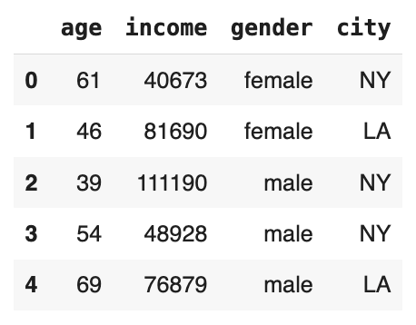
The above code created a small dataset containing size=20 instances of citizens’ data with randomly generated values and categories, depending on the attribute type. Concretely, each citizen is described by two numerical features — age and income — two categorical attributes — gender and city —, and one binary target label with no specific semantics in this example (think, for example, of interpreting it as whether or not the citizen would vote for a certain political party).
Before starting the feature engineering pipeline, we will separate the label from the rest of the features and define two Python lists containing the names of the numeric and categorical features, respectively. These lists will play a key role when using a ColumnTransformer to apply customized data transformations that vary from one feature to another.
|
X = df.drop(‘label’, axis=1) y = df[‘label’] numeric_features = [‘age’, ‘income’] categorical_features = [‘gender’, ‘city’] |
This is what the features look like:
Next, we define the preprocessing steps, namely, two parallel pipelines (one for each subset of attributes identified earlier), joined by a column transformer.
|
numeric_transformer = Pipeline(steps=[ (‘scaler’, StandardScaler()) ]) categorical_transformer = Pipeline(steps=[ (‘encoder’, OneHotEncoder(handle_unknown=‘ignore’)) ]) # The two “atomic” pipelines are combined preprocessor = ColumnTransformer( transformers=[ (‘num’, numeric_transformer, numeric_features), (‘cat’, categorical_transformer, categorical_features) ] ) |
Notice that the steps list inside each pipeline may contain one or several procedural stages to be applied in the pipeline. In this case, both pipelines are single-stage &mdash one of them applying standardization and the other applying one-hot encoding — but later on, we will define an overarching pipeline with multiple sequential stages in it.
Meanwhile, the ColumnTransformer object is where we have put both pipelines together via its transformers attribute, such that the pipelines are applied in parallel. All it takes is specifying here which features will be targeted by each of the two pipelines: that’s where the two previously defined lists of attribute names become handy.
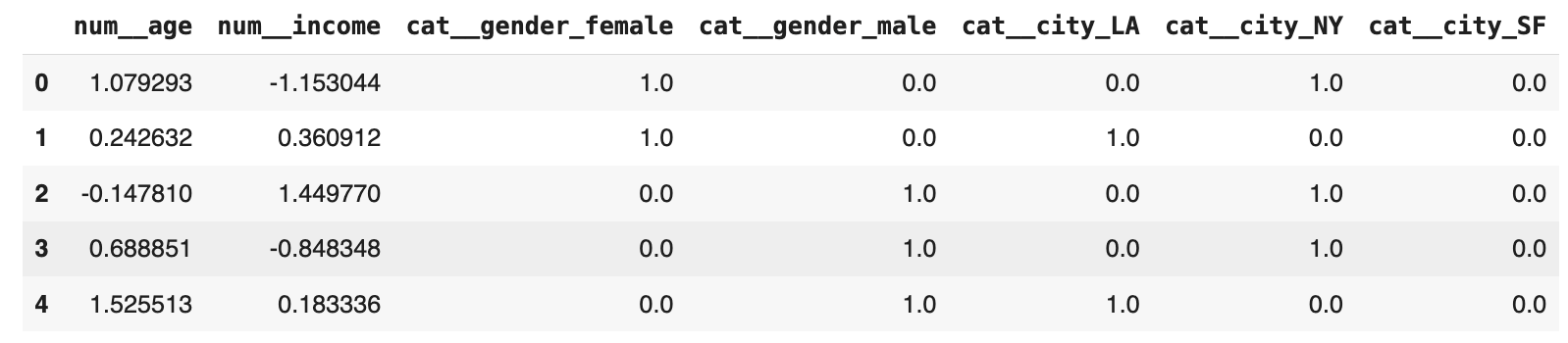
At this point, we can try out the combined feature engineering pipeline we just defined, and see what the data looks like after transformations (the resulting NumPy array is mapped onto a DataFrame for a more flashy visualization):
|
X_preprocessed = preprocessor.fit_transform(X) preprocessed_feature_names = preprocessor.get_feature_names_out() X_preprocessed_df = pd.DataFrame(X_preprocessed, columns=preprocessed_feature_names) print(“Preprocessed Data:”) X_preprocessed_df.head() |
Before finalizing, let me show you how to combine the feature engineering pipeline we created, named preprocessor, with the construction of a machine learning model for classification, e.g. a random forest, into an overarching pipeline, this time containing a sequence of two steps: feature engineering and machine learning modeling.
|
feng_pipeline = Pipeline(steps=[ (‘preprocessing’, preprocessor), (‘classifier’, RandomForestClassifier()) ]) feng_pipeline.fit(X, y) predictions = feng_pipeline.predict(X) print(predictions) |
Thanks to the use of NumPy arrays after preprocessing, the pipeline works seamlessly by passing these data structures to the random forest for training without the need for any data structure modifications.
Wrapping Up
This article showed how to use Scikit-learn’s Pipeline and Pandas’ ColumnTransformer objects, along with NumPy arrays, to perform advanced and customized feature engineering processes on datasets containing a variety of features of different types.