
Source: MachineLearningMastery.com
In this article, you will learn whether incorporating large language model embeddings as engineered features can meaningfully improve time series forecasting performance.
Topics we will cover include:
- Building a baseline forecasting model using only traditional time series features.
- Generating and reducing large language model embeddings from financial news headlines.
- Comparing model performance with and without embedding-based features.
Let’s get straight to it.
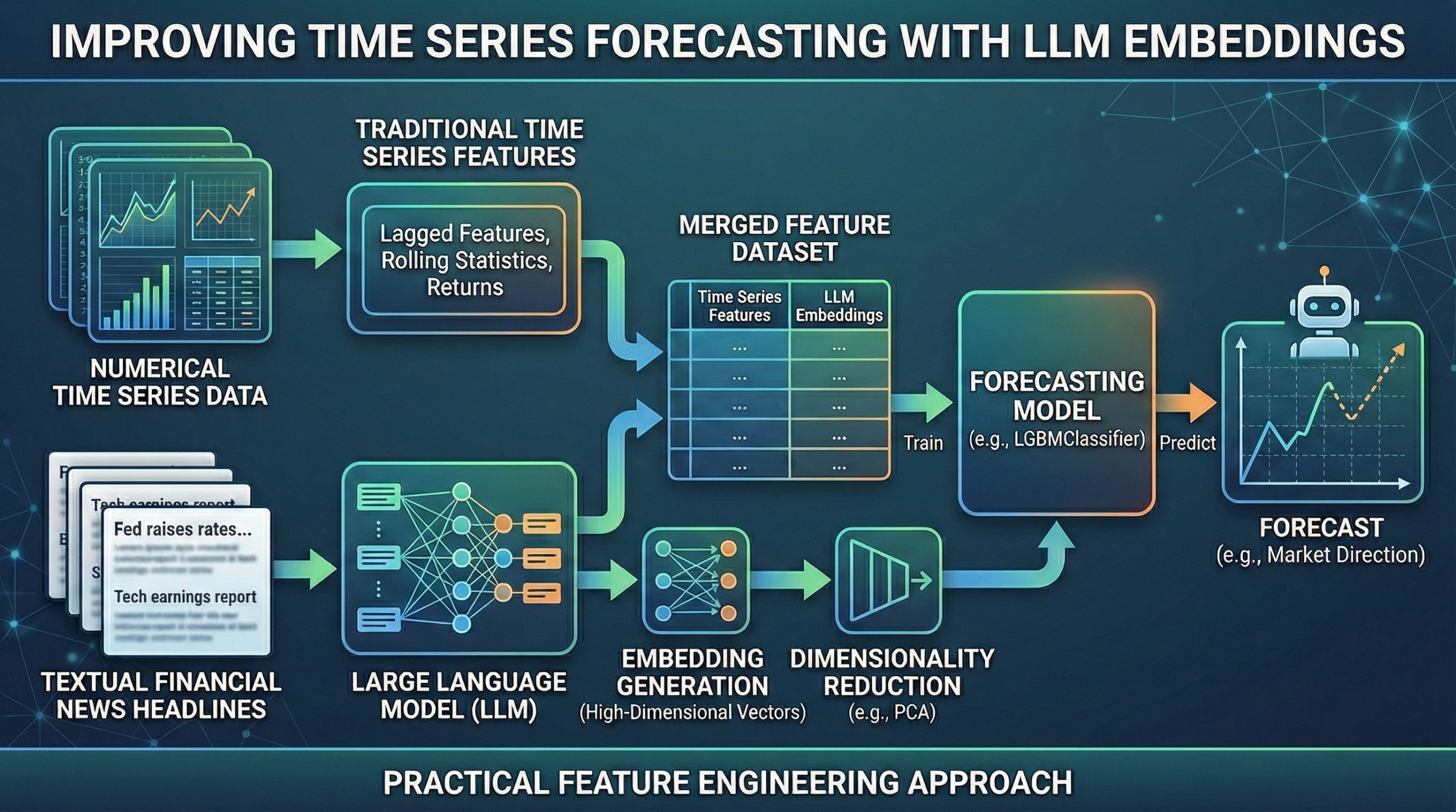
Can LLM Embeddings Improve Time Series Forecasting? A Practical Feature Engineering Approach (click to enlarge)
Image by Editor
Introduction
Using large language models (LLMs) — or their outputs, for that matter — for all kinds of machine learning-driven tasks, including predictive ones that were already being solved long before language models emerged, has become something of a trend. This naturally raises a question in the context of time series forecasting: does leveraging LLMs, for example by using LLM-generated embeddings engineered as additional features, really help improve the performance of models trained for time series forecasting?
Through a step-by-step practical example that encourages critical reflection, this article aims to address this pressing question about the usefulness of LLMs in predictive tasks such as forecasting the future.
LLM Embeddings for Improving Financial Time Series Forecasting: A Practical Walkthrough
We begin by importing the necessary modules and libraries for this example, in which we will create two versions of a dataset for training forecasting models: one containing only time series-related features, and another that also incorporates LLM-generated embeddings derived from a different (but somewhat causally related) dataset.
The two datasets used are:
- Dow Jones Industrial Average: daily adjusted closing prices for 30 large-cap U.S. companies in the DJIA. We will retrieve this dataset using the yfinance library.
Combined_News_DJIAheadlines: daily top-25 financial news headlines, largely including companies listed in the DJIA.
|
import pandas as pd import numpy as np import yfinance as yf from sentence_transformers import SentenceTransformer from sklearn.decomposition import PCA from sklearn.metrics import accuracy_score from lightgbm import LGBMClassifier |
The next code excerpt loads the first dataset and applies simple feature engineering to add lagged features and rolling statistics — a common practice in time series preprocessing to better capture meaningful signal patterns for downstream forecasting tasks:
|
1 2 3 4 5 6 7 8 9 10 11 12 13 14 15 16 17 18 |
ticker = “^DJI” df_price = yf.download(ticker, start=“2008-01-01”, end=“2016-12-31”) df_price = df_price[[“Close”]] df_price[“return”] = df_price[“Close”].pct_change() df_price[“target”] = (df_price[“return”].shift(–1) > 0).astype(int) df_price = df_price.dropna() df_price.head() # Adding lagged and rolling average features for lag in [1, 2, 3, 5]: df_price[f“lag_{lag}”] = df_price[“return”].shift(lag) df_price[“roll_mean_5”] = df_price[“return”].rolling(5).mean() df_price[“roll_std_5”] = df_price[“return”].rolling(5).std() df_price = df_price.dropna() |
Take note of the prefixes used in the names of these engineered features, as we will refer back to them later.
Next, we load the news headlines dataset and combine the daily headlines into a single text column. This is a deliberately simple approach for illustration purposes, and it could be made far more sophisticated — for example, by filtering headlines more strictly for DJIA-related content.
|
1 2 3 4 5 6 7 8 9 10 11 12 13 14 15 16 17 |
df_news = pd.read_csv( “https://raw.githubusercontent.com/gakudo-ai/open-datasets/refs/heads/main/Combined_News_DJIA.csv” ) df_news.columns = df_news.columns.str.strip() df_news[“Date”] = pd.to_datetime(df_news[“Date”], dayfirst=True) headline_cols = [c for c in df_news.columns if c.startswith(“Top”)] df_news[headline_cols] = df_news[headline_cols].fillna(“”) df_news[“combined”] = df_news[headline_cols].apply( lambda row: ” “.join([str(x) for x in row if str(x).strip() != “”]), axis=1 ) df_news[“combined”].head() |
The following helper function is not strictly necessary, but it is useful for removing awkward characters resulting from the fact that some strings in this dataset were originally byte-encoded:
|
1 2 3 4 5 6 7 8 9 10 11 12 13 14 15 16 17 18 19 20 |
import ast def clean_bytes_text(x): “”“ Convert byte-like strings (b’…’) to normal text ““” if isinstance(x, str): try: evaluated_value = ast.literal_eval(x) if isinstance(evaluated_value, bytes): return evaluated_value.decode(‘utf-8’) else: return str(evaluated_value) except (ValueError, SyntaxError): if x.startswith(“b”): return x.strip(“b'””) return x return x df_news[“combined”] = df_news[“combined”].apply(clean_bytes_text) |
We now use a pre-trained sentence transformer model to generate embeddings, passing the concatenated news headlines in the "combined" column as input:
|
model = SentenceTransformer(“all-MiniLM-L6-v2”) embeddings = model.encode( df_news[“combined”].tolist(), show_progress_bar=True ) |
To reduce the risk of overfitting and limit the dimensionality of the embedding space, we apply principal component analysis (PCA):
|
pca = PCA(n_components=20) embeddings_reduced = pca.fit_transform(embeddings) emb_df = pd.DataFrame( embeddings_reduced, index=df_news[“Date”], columns=[f“emb_{i}” for i in range(20)] ) |
Now comes the most intricate part of the process: merging the time series features with the generated embedding dimensions into a single dataset. The procedure involves preparing df_price for merging by cleaning column names, flattening potential MultiIndex columns, and ensuring that 'Date' is represented as a single-level column. The result is then merged with emb_df on 'Date'.
|
1 2 3 4 5 6 7 8 9 10 11 12 13 14 15 16 17 18 19 20 21 22 23 24 25 26 27 28 |
emb_df = emb_df.copy() emb_df.reset_index(inplace=True) emb_df.rename(columns={emb_df.columns[0]: “Date”}, inplace=True) if ‘level_0’ in df_price.columns: df_price = df_price.drop(columns=[‘level_0’]) if ‘index’ in df_price.columns: df_price = df_price.drop(columns=[‘index’]) df_price_cleaned = df_price.reset_index() if isinstance(df_price_cleaned.columns, pd.MultiIndex): new_cols = [] for col in df_price_cleaned.columns: if col[0] == ‘Date’: new_cols.append(‘Date’) elif isinstance(col, tuple) and col[1] != ”: new_cols.append(col[1]) else: new_cols.append(col[0]) df_price_cleaned.columns = new_cols if ‘Ticker’ in df_price_cleaned.columns: df_price_cleaned = df_price_cleaned.drop(columns=[‘Ticker’]) df_price_cleaned[‘Date’] = pd.to_datetime(df_price_cleaned[‘Date’]) df = pd.merge(df_price_cleaned, emb_df, on=“Date”, how=“inner”) |
Recall the prefixes used for the time series features. We now separate the column names into two groups: those related to traditional time series attributes and those corresponding to LLM embeddings.
|
emb_features = [col for col in df.columns if “emb_” in col] ts_features = [col for col in df.columns if “lag_” in col or “roll_” in col] |
With these feature groups defined, we move to the final stage: training two forecasting models. The first is a baseline model using only time series features, while the second combines these with embedding-based features.
|
# IMPORTANT: set ‘Date’ as the DataFrame index for proper time series splitting df = df.set_index(‘Date’) train = df[df.index < “2014-01-01”] # Splitting threshold test = df[df.index >= “2014-01-01”] X_train_base = train[ts_features] X_test_base = test[ts_features] X_train_full = train[ts_features + emb_features] X_test_full = test[ts_features + emb_features] y_train = train[“target”] y_test = test[“target”] |
Finally, we train the two models and compare their performance.
|
# Baseline model: no LLM embeddings model_base = LGBMClassifier(random_state=42) model_base.fit(X_train_base, y_train) pred_base = model_base.predict(X_test_base) acc_base = accuracy_score(y_test, pred_base) print(“Baseline Accuracy:”, acc_base) |
Baseline Accuracy: 0.5.
|
# Full model with LLM embeddings model_full = LGBMClassifier(random_state=42) model_full.fit(X_train_full, y_train) pred_full = model_full.predict(X_test_full) acc_full = accuracy_score(y_test, pred_full) print(“With Embeddings Accuracy:”, acc_full) |
Full Model Accuracy: 0.5047619047619047.
Verdict: Can LLMs Improve Time Series Forecasting?
Interestingly, the full model’s accuracy is only marginally higher than the baseline — effectively identical in practical terms. The results are therefore inconclusive. You may also experiment with slightly adjusting the threshold date (January 1, 2014) used to split the dataset into training and test sets and observe how sensitive the results can be. In some cases, performance differences may become even more volatile.
This naturally leads us to a nuanced answer to the question posed at the beginning of the article.
Can LLM embeddings improve time series forecasting?
The answer, perhaps unsurprisingly, is: it depends. While LLM embeddings integrated through feature engineering — sometimes referred to as LLM-based time series forecasting — can be promising in specific contexts, they are far from a universal replacement for traditional forecasting approaches based purely on temporal features.
Some recent studies suggest that although LLMs can improve performance in particularly data-scarce or text-rich scenarios, they often add limited value — and may even underperform — in environments characterized by high-frequency, complex numerical, or highly erratic data. A sensible strategy is to evaluate embedding-augmented forecasting models across multiple experimental settings and time splits, assessing whether improvements over a well-defined baseline are consistent and statistically meaningful.
In short, LLM embeddings may add value in certain forecasting scenarios — but careful experimentation, robust validation, and domain awareness remain essential.