Training a Model with Limited Memory using Mixed Precision and Gradient Checkpointing

Source: MachineLearningMastery.com

Training a language model is memory-intensive, not only because the model itself is large but also because the long sequences in the training data batches. Training a model with limited memory is challenging. In this article, you will learn techniques that enable model training in memory-constrained environments. In particular, you will learn about:

Low-precision floating-point numbers and mixed-precision training
Using gradient checkpointing

Let’s get started!

Training a Model with Limited Memory using Mixed Precision and Gradient Checkpointing
Photo by Meduana. Some rights reserved.

Overview

This article is divided into three parts; they are:

Floating-point Numbers
Automatic Mixed Precision Training
Gradient Checkpointing

Let’s get started!

Floating-Point Numbers

The default data type in PyTorch is the IEEE 754 32-bit floating-point format, also known as single precision. It is not the only floating-point type you can use. For example, most CPUs support 64-bit double-precision floating-point, and GPUs often support half-precision floating-point as well. The table below lists some floating-point types:

Data Type	PyTorch Type	Total Bits	Sign Bit	Exponent Bits	Mantissa Bits	Min Value	Max Value	eps
IEEE 754 double precision	`torch.float64`	64	1	11	52	-1.79769e+308	1.79769e+308	2.22045e-16
IEEE 754 single precision	`torch.float32`	32	1	8	23	-3.40282e+38	3.40282e+38	1.19209e-07
IEEE 754 half precision	`torch.float16`	16	1	5	10	-65504	65504	0.000976562
bf16	`torch.bfloat16`	16	1	8	7	-3.38953e+38	3.38953e+38	0.0078125
fp8 (e4m3)	`torch.float8_e4m3fn`	8	1	4	3	-448	448	0.125
fp8 (e5m2)	`torch.float8_e5m2`	8	1	5	2	-57344	57344	0.25
fp8 (e8m0)	`torch.float8_e8m0fnu`	8	1	8	0	1.70141e+38	5.87747e-39	1.0
fp6 (e3m2)		6	1	3	2	-28	28	0.25
fp6 (e2m3)		6	1	2	3	-7.5	7.5	0.125
fp4 (e2m1)		4	1	2	1	-6	6

Floating-point numbers are binary representations of real numbers. Each consists of a sign bit, several bits for the exponent, and several bits for the mantissa. They are laid out as shown in the figure below. When sorted by their binary representation, floating-point numbers retain their order by real-number value.

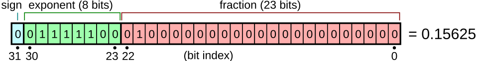
Floating-point number representation. Figure from Wikimedia.

Different floating-point types have different ranges and precisions. Not all types are supported by all hardware. For example, fp4 is only supported in Nvidia’s Blackwell architecture. PyTorch supports only a few data types. You can run the following code to print information about various floating-point types:

import torch

from tabulate import tabulate

# float types:

float_types = [

torch.float64,

torch.float32,

torch.float16,

torch.bfloat16,

torch.float8_e4m3fn,

torch.float8_e5m2,

torch.float8_e8m0fnu,

]

# collect finfo for each type

table = []

for dtype in float_types:

info = torch.finfo(dtype)

try:

typename = info.dtype

except:

typename = str(dtype)

table.append([typename, info.max, info.min, info.smallest_normal, info.eps])

headers = [‘data type’, ‘max’, ‘min’, ‘smallest normal’, ‘eps’]

print(tabulate(table, headers=headers))

Pay attention to the min and max values for each type, as well as the eps value. The min and max values indicate the range a type can support (the dynamic range). If you train a model with such a type, but the model weights exceed this range, you will get overflow or underflow, usually causing the model to output NaN or Inf. The eps value is the smallest positive number such that the type can differentiate between 1+eps and 1. This is a metric for precision. If your model’s gradient updates are smaller than eps, you will likely observe the vanishing gradient problem.

Therefore, float32 is a good default choice for deep learning: it has a wide dynamic range and high precision. However, each float32 number requires 4 bytes of memory. As a compromise, you can use float16 to save memory, but you are likely to encounter overflow or underflow issues since the dynamic range is much smaller.

The Google Brain team identified this problem and proposed bfloat16, a 16-bit floating-point format with the same dynamic range as float32. As a trade-off, the precision is an order of magnitude worse than float16. It turns out that dynamic range is more important than precision for deep learning, making bfloat16 highly useful.

When you create a tensor in PyTorch, you can specify the data type. For example:

x = torch.tensor([1.0, 2.0, 3.0], dtype=torch.float16)

print(x)

There is a straightforward way to change the default to a different type, such as bfloat16. This is handy for model training. All you need to do is set the following line before you create any model or optimizer:

# set default dtype to bfloat16

torch.set_default_dtype(torch.bfloat16)

Just by doing this, you force all your model weights and gradients to be bfloat16 type. This saves half of the memory. In the previous article, you were advised to set the batch size to 8 to fit a GPU with only 12GB of VRAM. With bfloat16, you should be able to set the batch size to 16.

Note that attempting to use 8-bit float or lower-precision types may not work. This is because you need hardware support and PyTorch to perform the corresponding mathematical operations. You can try the following code (requires a CUDA device) and find that you will need extra effort to operate on 8-bit float:

dtype = torch.float8_e4m3fn

# Define a tensor with float8 will see

# NotImplementedError: “normal_kernel_cuda” not implemented for ‘Float8_e4m3fn’

x = torch.randn(16, 16, dtype=dtype, device=“cuda”)

# Create in float32 and convert to float8 works

x = torch.randn(16, 16, device=“cuda”).to(dtype)

# But matmul is not supported. You will see

# NotImplementedError: “addmm_cuda” not implemented for ‘Float8_e4m3fn’

y = x @ x.T

# The correct way to run matrix multiplication on 8-bit float

y = torch._scaled_mm(x, x.T, out_dtype=dtype,

scale_a=torch.tensor(1.0, device=“cuda”),

scale_b=torch.tensor(1.0, device=“cuda”))

print(y)

Automatic Mixed Precision Training

Training a model with float16 may encounter issues because not all operations should be performed at lower precision. For example, matrix multiplication is robust in lower precision, but reduction operations, pooling, and some activation functions require float32.

You can set the data type manually for each component of your model, but this is tedious because you must convert data types between components. A better solution is to use automatic mixed precision training in PyTorch.

PyTorch has a sub-library torch.amp that can automatically cast the data type based on the operation. Not all operations are carried out in the same floating-point type. If the operation is known to be robust at lower precision, this library will cast the tensors to that precision before running the operation. Hence the name “mixed precision”. Using lower precision may not only save memory but also speed up training. Some GPUs can run float16 operations at twice the speed of float32.

When you train a model with torch.amp, all you need to do is run your forward pass under the context of torch.amp.autocast(). Typically, you will also use a GradScaler to handle gradient scaling. This is necessary because under low precision, you may encounter vanishing gradients due to the limited precision of your floating-point type. The GradScaler scales the gradient before the backward pass to prevent loss of gradient flow. During the backward pass, you should scale the gradient back for accurate updates. This process can be cumbersome because you need to determine the correct scale factor, which the GradScaler handles for you.

Compared to the training loop from the previous article, below is how you typically use torch.amp to train a model:

...

# Check if mixed precision training is supported

assert torch.amp.autocast_mode.is_autocast_available(“cuda”)

# Creates a GradScaler before the training loop

scaler = torch.amp.GradScaler(“cuda”, enabled=True)

# start training

for epoch in range(begin_epoch, epochs):

pbar = tqdm.tqdm(dataloader, desc=f“Epoch {epoch+1}/{epochs}”)

for batch_id, batch in enumerate(pbar):

# get batched data

input_ids, target_ids = batch

# create attention mask: causal mask + padding mask

attn_mask = create_causal_mask(input_ids.shape[1], device) +

create_padding_mask(input_ids, PAD_TOKEN_ID, device)

# with autocasting to bfloat16, run the forward pass

with torch.autocast(device_type=“cuda”, dtype=torch.bfloat16):

logits = model(input_ids, attn_mask)

loss = loss_fn(logits.view(–1, logits.size(–1)), target_ids.view(–1))

# backward with loss, scaled by the GradScaler

optimizer.zero_grad()

scaler.scale(loss).backward()

# step the optimizer and check if the scale has been updated

scaler.step(optimizer)

old_scale = scaler.get_scale()

scaler.update()

if scaler.get_scale() < old_scale:

scheduler.step()

pbar.set_postfix(loss=loss.item())

pbar.update(1)

pbar.close()

Using AMP autocasting is straightforward: keep the model’s default precision at float32, then wrap the forward pass and loss computation with torch.autocast(). Under this context, all supported operations will run in the specified data type.

Once you have the loss, let the GradScaler handle the backward pass. It will scale up the loss and update the model’s gradients. However, this may cause issues if the scaling is too large, resulting in NaN or Inf gradients. Therefore, use scaler.step(optimizer) to step the optimizer, which verifies the gradients before executing the optimizer step. If GradScaler decides not to step the optimizer, it will reduce the scale factor when update() is called. Check whether the scale has been updated to determine if you should step the scheduler.

Since the backward pass uses scaled loss, if you use gradient clipping, you should unscale the gradients before clipping. Here’s how to do it:

...

# backward with loss, scaled by the GradScaler

optimizer.zero_grad()

scaler.scale(loss).backward()

# unscaled the gradients and apply gradient clipping

scaler.unscale_(optimizer)

torch.nn.utils.clip_grad_norm_(model.parameters(), 1.0)

# step the optimizer and check if the scale has been updated

scaler.step(optimizer)

old_scale = scaler.get_scale()

scaler.update()

if scaler.get_scale() < old_scale:

scheduler.step()

Normally, you don’t need to call scaler.unscale_() manually since it’s part of the scaler.step(optimizer) call. However, you must do so when applying gradient clipping so that the clipping function can observe the actual gradients.

Autocasting is automatic, but the GradScaler maintains a state to track the scale factor. Therefore, when you checkpoint your model, you should also save the scaler.state_dict(), just as you would save the optimizer state:

...

# Loading checkpoint

checkpoint = torch.load(“training_checkpoint.pth”)

model.load_state_dict(checkpoint[“model”])

optimizer.load_state_dict(checkpoint[“optimizer”])

scheduler.load_state_dict(checkpoint[“scheduler”])

scaler.load_state_dict(checkpoint[“scaler”])

# Saving checkpoint

torch.save({

“model”: model.state_dict(),

“optimizer”: optimizer.state_dict(),

“scheduler”: scheduler.state_dict(),

“scaler”: scaler.state_dict(),

}, f“training_checkpoint.pth”)

Gradient Checkpointing

When you train a model with half precision, you use half the memory compared to 32-bit float. With mixed-precision training, you may use slightly more memory because not all operations run at lower precision.

If you still encounter memory issues, another technique trades time for memory: gradient checkpointing. Recall that in deep learning, for a function $y=f(mathbb{u})$ and $mathbb{u}=g(mathbb{x}))$, then

$$
frac{partial y}{partial mathbb{x}} = big(frac{partial mathbb{u}}{partial mathbb{x}}big)^top frac{partial y}{partial mathbb{u}}
$$

where $y$ is a scalar (usually the loss metric), and $mathbb{u}$ and $mathbb{x}$ are vectors. The term $frac{partial mathbb{u}}{partial mathbb{x}}$ is the Jacobian matrix of $mathbb{u}$ with respect to $mathbb{x}$.

The gradient $frac{partial y}{partial mathbb{x}}$ is needed to update $mathbb{x}$ but depends on $frac{partial y}{partial mathbb{u}}$. Normally, when you run the forward pass, all intermediate results such as $mathbb{u}$ are stored in memory so that when you run the backward pass, you can readily compute the gradient $frac{partial y}{partial mathbb{u}}$. However, this requires substantial memory for deep networks.

Gradient checkpointing discards some intermediate results. As long as you know $mathbb{u}=g(mathbb{x})$, you can recompute $mathbb{u}$ from $mathbb{x}$ during the backward pass. This way, you don’t need to store $mathbb{u}$ in memory, but you must compute $mathbb{u}$ twice: once for the forward pass and once for the backward pass.

You can decide which intermediate results to discard. Applying gradient checkpointing to every two operations still requires storing many intermediate results. Applying it to larger blocks saves more memory.

Referring to the model from the previous article, you can wrap every transformer block with gradient checkpointing:

...

class LlamaModel(nn.Module):

def __init__(self, config: LlamaConfig) -> None:

super().__init__()

self.rotary_emb = RotaryPositionEncoding(

config.hidden_size // config.num_attention_heads,

config.max_position_embeddings,

)

self.embed_tokens = nn.Embedding(config.vocab_size, config.hidden_size)

self.layers = nn.ModuleList([LlamaDecoderLayer(config) for _ in range(config.num_hidden_layers)])

self.norm = nn.RMSNorm(config.hidden_size, eps=1e–5)

def forward(self, input_ids: Tensor, attn_mask: Tensor) -> Tensor:

# Convert input token IDs to embeddings

hidden_states = self.embed_tokens(input_ids)

# Process through all transformer layers, then the final norm layer

for layer in self.layers:

# Previously:

# hidden_states = layer(hidden_states, rope=self.rotary_emb, attn_mask=attn_mask)

hidden_states = torch.utils.checkpoint.checkpoint(layer, hidden_states, self.rotary_emb, attn_mask)

hidden_states = self.norm(hidden_states)

# Return the final hidden states

return hidden_states

Only one line of code needs to change: in the for-loop under the forward() function, instead of calling the transformer block directly, use torch.utils.checkpoint.checkpoint(). This runs the forward pass with gradient checkpointing, discarding all intermediate results and retaining only the block’s input and output. During the backward pass, the intermediate results are temporarily recomputed using the input.

Summary

In this article, you learned techniques for training a language model with limited memory. Specifically, you learned that:

Several types of floating-point numbers exist, with some using less memory than others.
Mixed-precision training automatically uses lower-precision floating-point numbers without sacrificing accuracy on critical operations.
Gradient checkpointing trades time for memory during training.