Source: MarkTechPost
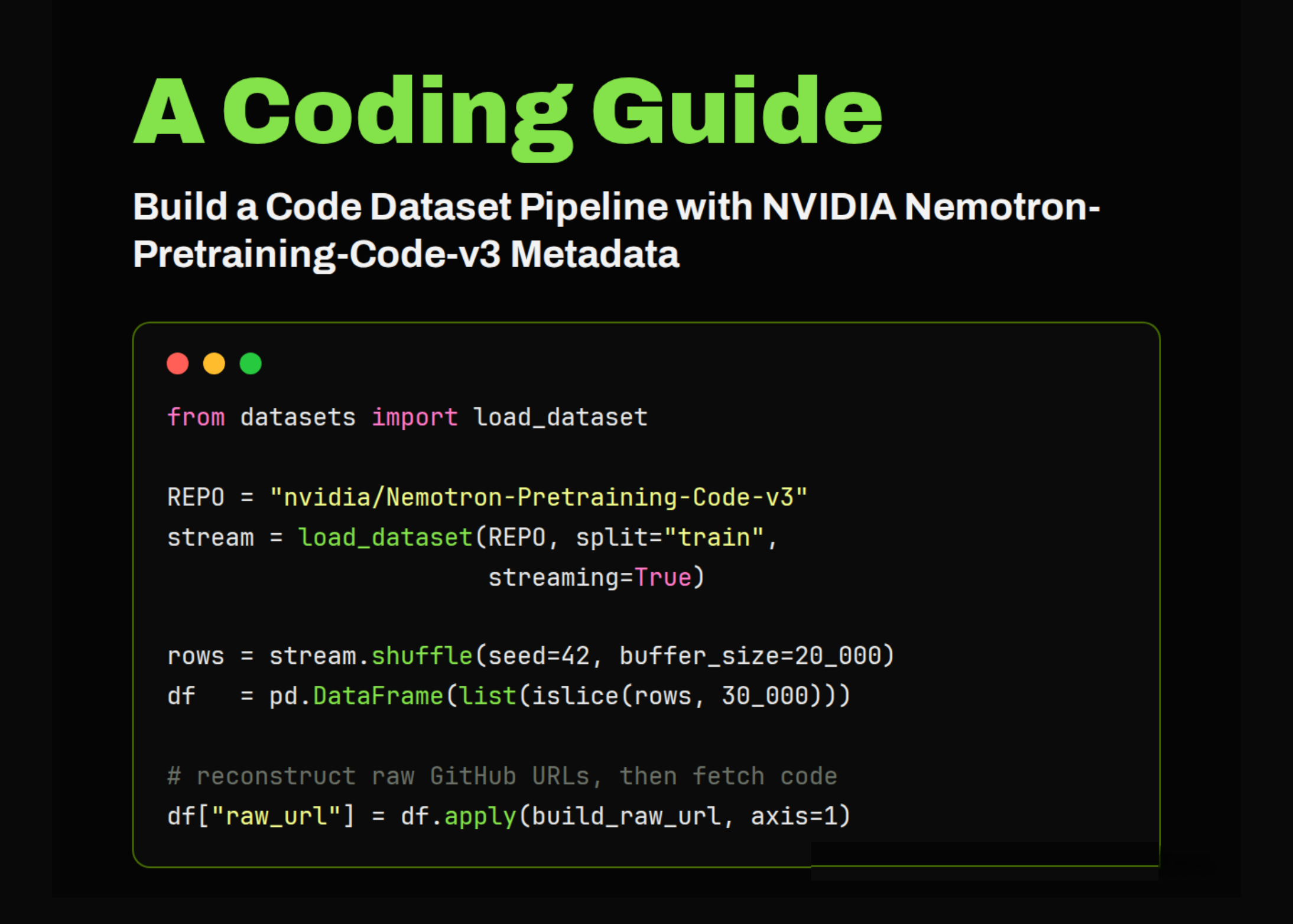
In this tutorial, we work with NVIDIA’s Nemotron-Pretraining-Code-v3 dataset as a large-scale metadata index for code pretraining research. Instead of downloading the full multi-gigabyte dataset, we stream it, inspect its schema, and build a manageable sample for analysis. We then explore the dataset by studying languages, file extensions, repository frequency, and directory depth, which helps us understand how the index is structured. After that, we reconstruct the raw GitHub URLs from the metadata, attempt to fetch the actual source files, and estimate the token scale of the fetched code. By the end of the workflow, we create a reusable filtered sample and save processed outputs for further experimentation.
Streaming the NVIDIA Nemotron-Pretraining-Code-v3 Dataset and Inspecting Its Schema
!pip -q install -U "datasets>=2.19" huggingface_hub tiktoken pyarrow 2>/dev/null import os, io, time, itertools, collections, textwrap, math import pandas as pd import requests import matplotlib.pyplot as plt from datasets import load_dataset, get_dataset_config_names REPO_ID = "nvidia/Nemotron-Pretraining-Code-v3" pd.set_option("display.max_colwidth", 80) configs = get_dataset_config_names(REPO_ID) CONFIG = configs[0] print(f"Configs available : {configs}") print(f"Using config : {CONFIG}") stream = load_dataset(REPO_ID, CONFIG, split="train", streaming=True) print("nFeatures / schema:") print(stream.features) print("nFirst raw record:") print(next(iter(stream)))We set up the Colab environment by installing the required libraries and importing the tools needed for dataset streaming, analysis, and visualization. We define the NVIDIA Nemotron-Pretraining-Code-v3 dataset ID, discover the available dataset configuration, and load the training split in streaming mode. We also inspect the dataset schema and print the first record to understand the structure before conducting deeper analysis.
Building a Shuffled Sample and Analyzing Code Metadata Features
N_SAMPLE = 30_000 shuffled = stream.shuffle(seed=42, buffer_size=20_000) t0 = time.time() rows = list(itertools.islice(shuffled, N_SAMPLE)) df = pd.DataFrame(rows) print(f"nPulled {len(df):,} rows in {time.time()-t0:,.1f}s") print(df.head(10)) print("nColumns:", list(df.columns), "| memory:", f"{df.memory_usage(deep=True).sum()/1e6:,.1f} MB") df["ext"] = df["rel_path"].str.extract(r".([A-Za-z0-9_]+)$")[0].str.lower() df["depth"] = df["rel_path"].str.count("https://www.marktechpost.com/") df["fname"] = df["rel_path"].str.rsplit("https://www.marktechpost.com/", n=1).str[-1] print("n--- Top 15 languages (sample) ---") lang_counts = df["language"].value_counts() print(lang_counts.head(15)) print("n--- Top 15 file extensions (sample) ---") print(df["ext"].value_counts().head(15)) print("n--- Most frequent repositories (sample) ---") print(df["repo"].value_counts().head(10)) print("n--- Path-depth summary ---") print(df["depth"].describe()) print(f"nUnique repos in sample : {df['repo'].nunique():,}") print(f"Unique languages : {df['language'].nunique():,}")We create a shuffled sample from the streamed dataset so that we do not rely only on the first clustered rows. We convert the sampled records into a Pandas DataFrame and derive useful features such as file extension, path depth, and file name. We then examine the most common languages, file extensions, repositories, and path-depth statistics to better understand the sampled metadata.
Visualizing Languages, File Extensions, Directory Depth, and Repository Frequency
fig, ax = plt.subplots(2, 2, figsize=(14, 9)) lang_counts.head(12).iloc[::-1].plot.barh(ax=ax[0, 0], color="#76b900") ax[0, 0].set_title("Top 12 languages (sample)"); ax[0, 0].set_xlabel("files") df["ext"].value_counts().head(12).iloc[::-1].plot.barh(ax=ax[0, 1], color="#5b8def") ax[0, 1].set_title("Top 12 file extensions (sample)"); ax[0, 1].set_xlabel("files") df["depth"].clip(upper=12).plot.hist(bins=range(0, 14), ax=ax[1, 0], color="#f4a261", edgecolor="white") ax[1, 0].set_title("Directory nesting depth"); ax[1, 0].set_xlabel("'/' count in path") (df["repo"].value_counts().head(10).iloc[::-1] .plot.barh(ax=ax[1, 1], color="#9b5de5")) ax[1, 1].set_title("Most common repos (sample)"); ax[1, 1].set_xlabel("files") plt.tight_layout(); plt.show()We visualize the main patterns found in the sampled metadata using multiple plots. We compare the top languages, top file extensions, directory nesting depth, and most frequent repositories in the sample. We use these charts to make the dataset easier to interpret and to quickly identify dominant structures inside the metadata index.
Reconstructing Raw GitHub URLs and Fetching Real Source Files
def raw_url(repo: str, commit_id: str, rel_path: str) -> str: from urllib.parse import quote return (f"https://raw.githubusercontent.com/{repo}/{commit_id}/" f"{quote(rel_path)}") df["raw_url"] = df.apply(lambda r: raw_url(r.repo, r.commit_id, r.rel_path), axis=1) print("nExample reconstructed URLs:") for u in df["raw_url"].head(5): print(" ", u) def fetch_code(url: str, max_bytes: int = 200_000, timeout: int = 10): try: resp = requests.get(url, timeout=timeout) if resp.status_code == 200 and len(resp.content) <= max_bytes: return resp.text return None except requests.RequestException: return None print("n--- Attempting to fetch a few real files ---") fetched, attempts = [], 0 for _, r in df.sample(frac=1, random_state=1).iterrows(): if len(fetched) >= 5: break attempts += 1 code = fetch_code(r["raw_url"]) status = "OK " if code else "MISS" print(f"[{status}] {r['language']:<12} {r['repo']}/{r['rel_path']}") if code: fetched.append({**r.to_dict(), "code": code, "n_chars": len(code)}) print(f"nFetched {len(fetched)} files in {attempts} attempts " f"(misses are normal — repos get deleted/renamed).") if fetched: ex = fetched[0] print(f"n----- PREVIEW: {ex['repo']}/{ex['rel_path']} ({ex['language']}) -----") print(textwrap.shorten(ex["code"].replace("n", " "), width=600, placeholder=" ...[truncated]"))We reconstruct raw GitHub URLs from the metadata: the repository name, commit ID, and relative file path. We then attempt to fetch a few real source files from GitHub, gracefully handling missing, deleted, private, or oversized files. We preview one successfully fetched file to see how the metadata index connects back to the actual code content.
Filtering Python Files, Estimating Token Scale, and Saving Outputs
TARGET_LANG = "Python" py_index = df[df["language"] == TARGET_LANG].copy() print(f"n{TARGET_LANG} files in sample: {len(py_index):,}") try: import tiktoken enc = tiktoken.get_encoding("cl100k_base") tok = lambda s: len(enc.encode(s, disallowed_special=())) except Exception: tok = lambda s: max(1, len(s) // 4) if fetched: toks = [tok(f["code"]) for f in fetched] print(f"Fetched-file tokens: total={sum(toks):,} " f"mean={sum(toks)/len(toks):,.0f}/file") TOTAL_FILES, TOTAL_TOKENS = 146_323_609, 173e9 print(f"nFull-dataset scale (per NVIDIA card): " f"{TOTAL_FILES:,} files ≈ {TOTAL_TOKENS/1e9:.0f}B tokens " f"(~{TOTAL_TOKENS/TOTAL_FILES:,.0f} tokens/file).") df.to_parquet("nemotron_code_v3_sample.parquet", index=False) if fetched: pd.DataFrame(fetched).to_json("nemotron_fetched_code.jsonl", orient="records", lines=True) print("nSaved: nemotron_code_v3_sample.parquet" + (", nemotron_fetched_code.jsonl" if fetched else "")) print("Done ✅")We filter the sampled index for Python files and estimate token counts for successfully fetched files. We use tiktoken when available and fall back on a simple character-based estimate when it is not. Also, we save the processed metadata sample and the fetched code outputs so we can reuse them later without having to stream the dataset again.
Conclusion
In conclusion, we built a practical end-to-end workflow to understand and use the Nemotron-Pretraining-Code-v3 metadata index. We learned how to stream the dataset efficiently, convert a sample into a DataFrame, perform exploratory analysis, visualize important patterns, and reconstruct GitHub file URLs from repository paths and commit identifiers. We also demonstrated how metadata can be traced back to the source code and how token estimation provides a sense of dataset scale.
Check out the Full Codes with Notebook. Also, feel free to follow us on Twitter and don’t forget to join our 150k+ ML SubReddit and Subscribe to our Newsletter. Wait! are you on telegram? now you can join us on telegram as well.
Need to partner with us for promoting your GitHub Repo OR Hugging Face Page OR Product Release OR Webinar etc.? Connect with us

Sana Hassan
Sana Hassan, a consulting intern at Marktechpost and dual-degree student at IIT Madras, is passionate about applying technology and AI to address real-world challenges. With a keen interest in solving practical problems, he brings a fresh perspective to the intersection of AI and real-life solutions.